# Macroeconomic Data: unemployment rate
unemp_rate <- rio::import("https://byuistats.github.io/timeseries/data/unemp_rate.csv")Time Series Homework: Chapter 1 Lesson 3
Eduardo Ramirez
Data
Questions
Question 1 - Estimating the Trend: Centered Moving Average (10 points)
Please plot the US Unemployment time series and superimpose the centered moving average series \(\hat{m}_{t}\) in the same graph. Don’t use an R command; rather, do it by coding \(\hat{m}_{t}\) like in Chapter 1: Lesson 3. Use the appropriate axis labels, units, and captions.
Answer
# Load packages
pacman::p_load("tsibble", "fable", "feasts", "tidyverse", "lubridate", "rio")


# Create a tsibble where the index variable is the year/month
unemp_rate_tsibble <- unemp_rate %>%
  mutate(date = ymd(date)) %>%
  as_tsibble(index = date)

# Calculate the Centred Moving Average (CMA)
unemp_rate_tsibble <- unemp_rate_tsibble %>%
  mutate(
    # Creating a new column 'm_hat', representing the centered moving average (CMA)
    m_hat = (
      # Math: (1/2) * x_{t-6}
      # Explanation: Fetches the value 6 time periods back and applies half-weight to it (beginning of the window)
      (1/2) * lag(value, 6) +

      # Math: x_{t-5}
      # Explanation: Fetches the value 5 time periods back with full weight
      lag(value, 5) +

      # Math: x_{t-4}
      lag(value, 4) +

      # Math: x_{t-3}
      lag(value, 3) +

      # Math: x_{t-2}
      lag(value, 2) +

      # Math: x_{t-1}
      # Explanation: Fetches the value 1 time period back with full weight
      lag(value, 1) +

      # Math: x_{t}
      # Explanation: Includes the value at the current time period
      value +

      # Math: x_{t+1}
      # Explanation: Fetches the value 1 time period forward with full weight
      lead(value, 1) +

      # Math: x_{t+2}
      lead(value, 2) +

      # Math: x_{t+3}
      lead(value, 3) +

      # Math: x_{t+4}
      lead(value, 4) +

      # Math: x_{t+5}
      # Explanation: Fetches the value 5 time periods forward with full weight
      lead(value, 5) +

      # Math: (1/2) * x_{t+6}
      # Explanation: Fetches the value 6 time periods forward and applies half-weight to it (end of the window)
      (1/2) * lead(value, 6)

    ) / 12  # Math: 1/12
            # Explanation: Divides the sum by 12 to compute the average over 12 time periods
  )


# Plot the CMA (centred moving average) and original data
plain_plot <- autoplot(unemp_rate_tsibble, .vars = m_hat) +
  labs(
    x = "Date",
    y = "Unemployment Rate (%)",
    title = "Centred Moving Average (CMA) of Unemployment Rate"
  ) +
  scale_y_continuous(limits = c(min(unemp_rate_tsibble$m_hat, na.rm = TRUE), max(unemp_rate_tsibble$m_hat, na.rm = TRUE))) +
  theme(plot.title = element_text(hjust = 0.5))

# Plot the original unemployment data with CMA overlay
fancy_plot <- autoplot(unemp_rate_tsibble, .vars = value) +
  labs(
    x = "Date",
    y = "Unemployment Rate (%)",
    title = "Monthly US Unemployment Rate with CMA"
  ) +
  geom_line(aes(x = date, y = m_hat), color = "#D55E00") +
  theme(plot.title = element_text(hjust = 0.5))

# Combine the two plots
plain_plot
Warning: Removed 12 rows containing missing values or values outside the scale range
(`geom_line()`).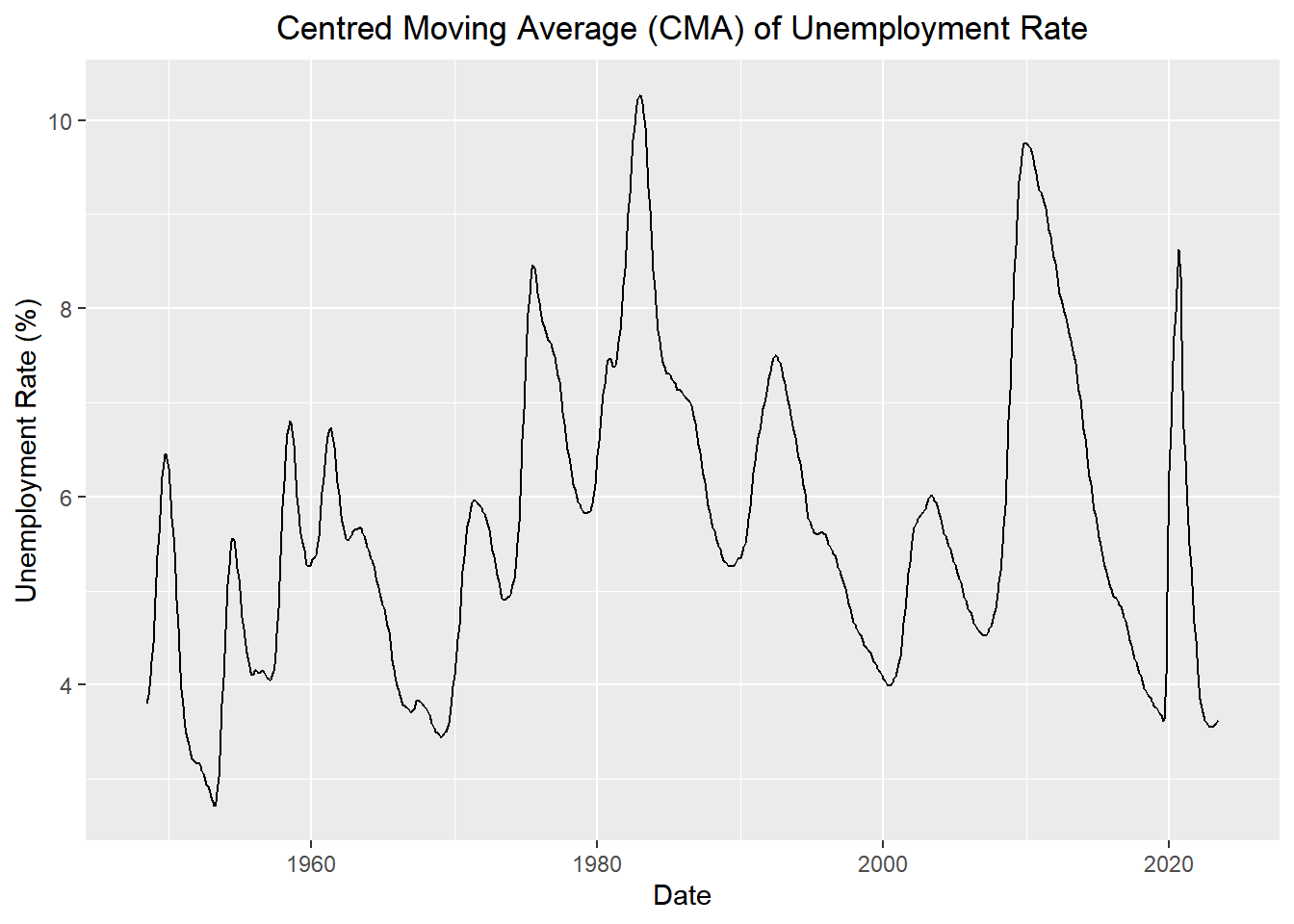
fancy_plotWarning: Removed 12 rows containing missing values or values outside the scale range
(`geom_line()`).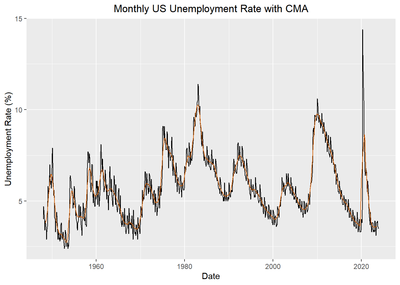
Question 2 - Seasonal Averages: Side-by-Side Box Plots by Month (10 points)
Please create a box plot to illustrate the monthly averages in the US Unemployment time series. Use the appropriate axis labels, units, and captions.
Question 3 - Seasonal Averages: Analysis (20 points)
a) Describe the seasonality of the US unemployment time series. Comment on the series’ periods of highest and lowest unemployment. Are there any notable outliers?
b) Please explain the patterns you found. Include information from your prior research on the series.

Rubric
| Criteria | Mastery (20) | Incomplete (0) |
| Question 1: Centered Moving Average | The student correctly employs the centering procedure to seasonally adjust the US unemployment series. | The student does not employ the centering procedure to seasonally adjust the US unemployment series. |
| Mastery (10) | Incomplete (0) | |
| Question 2: Box Plot | Creates a clear and well-constructed box plot that effectively illustrates seasonality in the US Unemployment time series. Labels both the x and y-axes, including appropriate units. Ensures clarity and accuracy in axis labeling, contributing to the overall understanding of the box plot. | There are mistakes in the plot. Fails to include any axis labels or units, resulting in an incomplete representation that lacks essential context. |
| Mastery (10) | Incomplete (0) | |
| Question 5a: Description | Provides an accurate description of the seasonality in the US Unemployment time series, capturing key patterns and trends effectively. Shows a good understanding of the recurring cycles. | Attempts to identify peaks and troughs but with significant inaccuracies or lack of clarity in the commentary. Shows a limited understanding of the variations. Fails to identify or comment on notable outliers, providing no insight into unusual data points in the US Unemployment time series. |
| Mastery (10) | Incomplete (0) | |
| Question 5b: Patterns | Shows understanding of the data to infer meaning in the seasonal averages. It’s clear the student did background research on the unemployment time series | Shows a lack of effort. It’s not clear the student understands the meaning of the data. |
| Total Points | 50 |