Level up your Tidy-ness

Putting it All Together

Here are two more data wrangling questions to test your skills. Try as best you can to work each step on your own before checking solutions.

The questions relate to the High School survey used in other examples.

# Load libraries and data

library(rio)
library(mosaic)
library(tidyverse)
library(car)

survey <- import('https://github.com/byuistats/Math221D_Cannon/raw/master/Data/HighSchoolSeniors_subset.csv') %>% tibble()

Telepaths, Gender and Sleep

Suppose we want to see who gets more sleep on non-school nights, males or females whose chosen superpower would be telepathy. Also, create a column that is the ratio of sleep hours on non-school nights to 8. This calculates the percent of recommended sleep on non-school nights.

Create a dataset that includes columns Gender, Superpower, Sleep_Hours_Non-Schoolnight, and the ratio of non-schoolnight sleep hours divided by 8, for Males and Females who choose Telepathy as their superpower.

# Your Code:

Solution

unique(survey$Superpower)

[1] "Telepathy"      "Invisibility"   "Fly"            "Freeze time"   
[5] "Super strength"

telepaths <- survey %>%
  select(Gender, Superpower, Sleep_Hours_Non_Schoolnight) %>%
  filter(Superpower=="Telepathy") %>%
  mutate(
    percent_of_recommended = Sleep_Hours_Non_Schoolnight / 8
  )

telepaths

# A tibble: 81 × 4
   Gender Superpower Sleep_Hours_Non_Schoolnight percent_of_recommended
   <chr>  <chr>                            <dbl>                  <dbl>
 1 Male   Telepathy                            7                  0.875
 2 Female Telepathy                            9                  1.12 
 3 Male   Telepathy                            9                  1.12 
 4 Female Telepathy                            8                  1    
 5 Female Telepathy                            9                  1.12 
 6 Male   Telepathy                           11                  1.38 
 7 Female Telepathy                           11                  1.38 
 8 Female Telepathy                            9                  1.12 
 9 Female Telepathy                            9                  1.12 
10 Female Telepathy                           10                  1.25 
# ℹ 71 more rows

Create a summary table comparing males and females whose preferred super power is telepathy that includes:

a. Mean, standard deviation, and sample size of Sleep Hours on non-school nights 
b. Mean, standard deviation, and sample size of the percent of recommended sleep

HINT: Use the unique() function to see what the options are for a given categorical variable.

# Your Code

Solution

telepaths %>%
  group_by(Gender) %>%
  summarise(
    mn_hrs = mean(Sleep_Hours_Non_Schoolnight),
    mn_percent_recommended = mean(percent_of_recommended),
    count = n()
  )

# A tibble: 2 × 4
  Gender mn_hrs mn_percent_recommended count
  <chr>   <dbl>                  <dbl> <int>
1 Female   8.73                   1.09    60
2 Male     8.19                   1.02    21

Vegetarians and Height

How many vegetarians say meat is their favorite food?

HINT: This can be done with a single filter statement

# Your Code:

Solution

survey %>%
  filter(Favorite_Food == "Meat",
         Vegetarian == "Yes")

# A tibble: 1 × 60
  Country Region DataYear ClassGrade Gender Ageyears Handed       Height_cm
  <chr>   <chr>     <int>      <int> <chr>     <dbl> <chr>            <dbl>
1 USA     NC         2022         11 Male         16 Right-Handed       178
# ℹ 52 more variables: Footlength_cm <dbl>, Armspan_cm <dbl>,
#   Languages_spoken <dbl>, Travel_to_School <chr>,
#   Travel_time_to_School <int>, Reaction_time <dbl>,
#   Score_in_memory_game <dbl>, Favourite_physical_activity <chr>,
#   Imprtance_reducing_pllutin <int>, Imprtance_recycling_rubbish <int>,
#   Imprtance_cnserving_water <int>, Imprtance_saving_energy <int>,
#   Imprtance_wning_cmputer <int>, Imprtance_Internet_access <int>, …

Compare mean, and standard deviation of heights between those who are vegetarian and those who aren’t. Include the number of respondents in your analysis.

Be sure to filter out any major outliers in heights first.

# Your Code:

Solution

survey %>%
  select(Height_cm, Vegetarian) %>%
  filter(Height_cm < 214,
         Height_cm > 100) %>%
  group_by(Vegetarian) %>%
  summarise(
    med_ht = median(Height_cm),
    mean_ht = mean(Height_cm),
    sd_ht = sd(Height_cm),
    count = n()
  )

# A tibble: 2 × 5
  Vegetarian med_ht mean_ht sd_ht count
  <chr>       <dbl>   <dbl> <dbl> <int>
1 No           170.    171.  10.8   285
2 Yes          163     162.  17.1    15

After removing outliers, it looks like vegetarians are shorter, on average.

# Bonus Boxplot:
veg <- survey %>%
  select(Height_cm, Vegetarian) %>%
  filter(Height_cm < 214,
         Height_cm > 100)


boxplot(veg$Height_cm ~ veg$Vegetarian, col = c(5,6), main = "Heights (cm) of Vegetarians and Non-Vegetarians", xlab="vegetarian", ylab = "Height (cm)")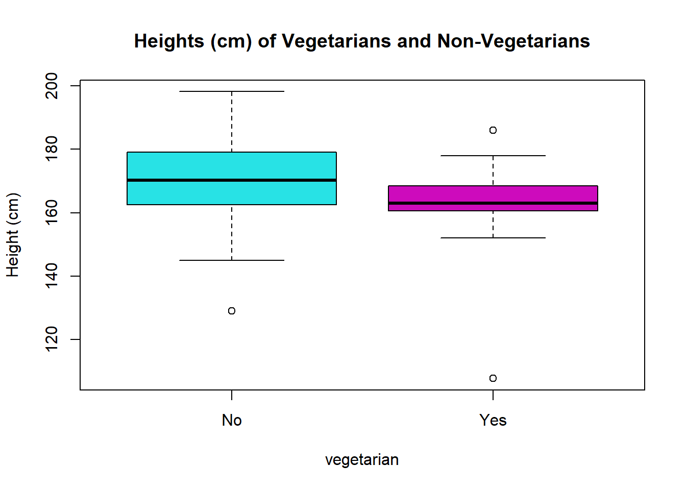

Create a dataset that:
1. Includes a column that is percent of recommended sleep (Sleep_Hours_Schoolnight divided by 8 using a mutate statement)
2. Includes only columns for Favourite_physical_activity, Reaction_time, percent_recommended_sleep (part a)
3. Includes only students whose favorite physical activity is Walking/Hiking, Basketball, Swimming, Soccer
4. Filters Reaction Times to be less than 1 second

# Your Code:

Solution

phys_act <- survey %>%
  mutate(
    pct_recommended_sleep = Sleep_Hours_Schoolnight / 8
  ) %>%
  filter(Favourite_physical_activity %in% c('Walking/Hiking', "Basketball", "Swimming", "Soccer"),
         Reaction_time < 1) %>%
  select(Favourite_physical_activity, Reaction_time, pct_recommended_sleep)

Use the clean dataset to:

Create a side-by-side boxplot for the percent of recommended sleep comparing favourite physical activity

# Your Code:

Solution

boxplot(phys_act$pct_recommended_sleep ~ phys_act$Favourite_physical_activity, xlab = "Favorite Physical Activity", ylab = "% Recommended Sleep on School Nights", main = "School Night Sleep by Favorite Physical Activity", col = c(2,3,4,5))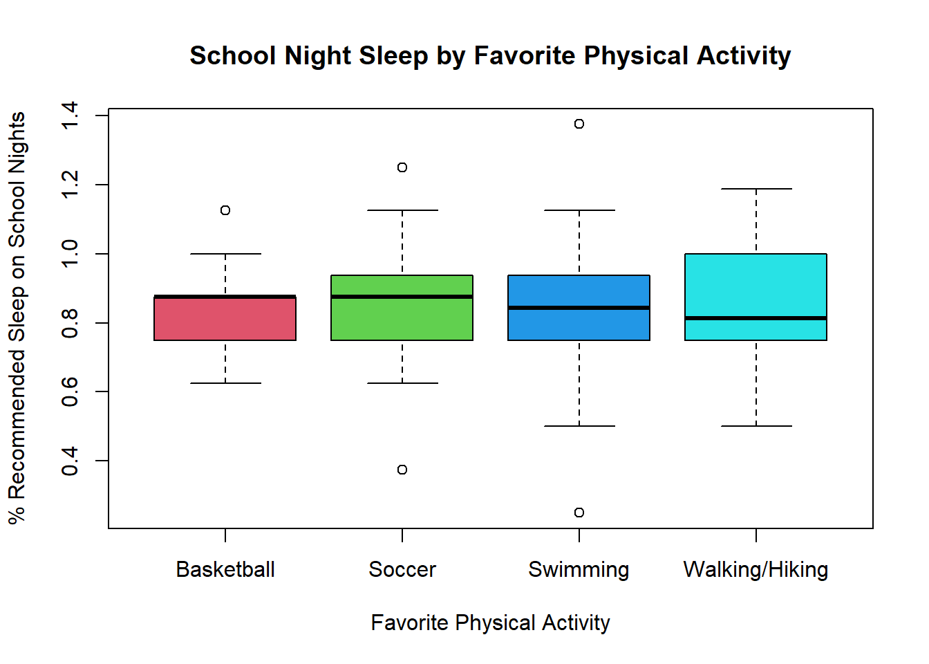

Create a side-by-side boxplot for the reaction times comparing favourite physical activity

# Your Code:

Solution

boxplot(phys_act$Reaction_time ~ phys_act$Favourite_physical_activity, xlab = "Favorite Physical Activity", ylab = "Reaction Time", main = "Reaction Time Results by Favorite Physical Activity", col = c(2,3,4,5))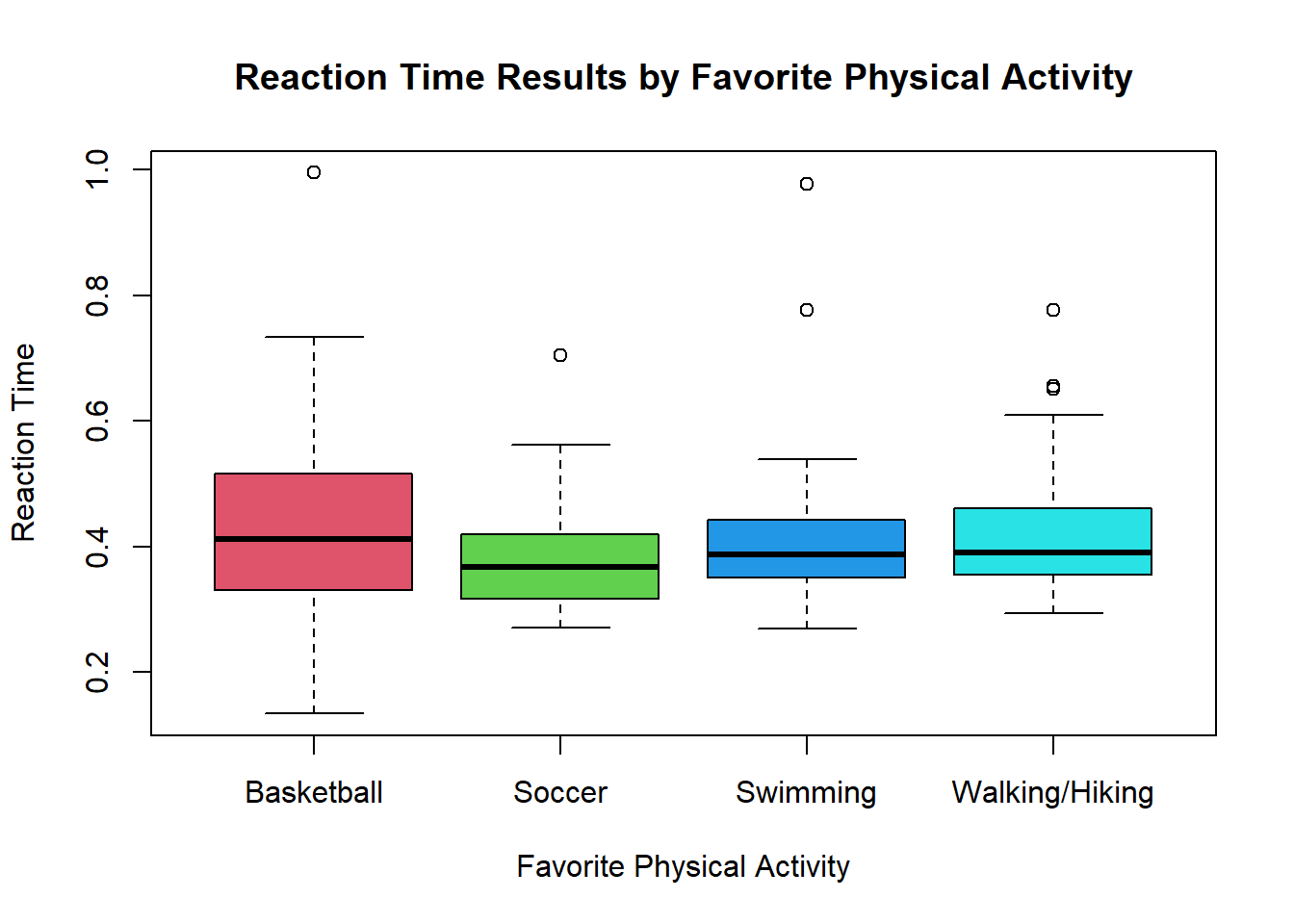

Which physical activity group has the quickest reaction time?